NATURAL LANGUAGE PROCESSING

Natural Language Processing (or NLP) is applying Machine Learning models to text and language. Teaching machines to understand what is said in spoken and written word is the focus of Natural Language Processing. Whenever you dictate something into your iPhone / Android device that is then converted to text, that’s an NLP algorithm in action.

You can also use NLP on a text review to predict if the review is a good one or a bad one. You can use NLP on an article to predict some categories of the articles you are trying to segment. You can use NLP on a book to predict the genre of the book. And it can go further, you can use NLP to build a machine translator or a speech recognition system, and in that last example you use classification algorithms to classify language. Speaking of classification algorithms, most of NLP algorithms are classification models, and they include Logistic Regression, Naive Bayes, CART which is a model based on decision trees, Maximum Entropy again related to Decision Trees, Hidden Markov Models which are models based on Markov processes.

A very well-known model in NLP is the Bag of Words model. It is a model used to preprocess the texts to classify before fitting the classification algorithms on the observations containing the texts.

In this part, you will understand and learn how to:

1.     Clean texts to prepare them for the Machine Learning models,

2.     Create a Bag of Words model,

3.     Apply Machine Learning models onto this Bag of Worlds model.

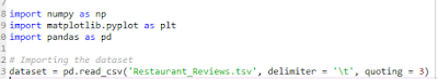
Importing the dataset:

So generally for importing the dataset we use extension of .csv file which stands for Comma separated values.But in the case NLP will will import .tsv file which stands for tab separated values because the columns separated by tab instead of commas.

For example:

In the following dataset it contains reviews of 1000 customer who visited the restaurant.So if we import this by using .csv file,then there arises a problem .Suppose consider the below review:

                         The food,amazing . ,1

The food and amazing are separated by commas which is considered as a new column which is not true.The whole review is supposed to be one column and the number 1 should be the second column.So to overcome this issue we use .tsv file in which the columns can be separated using space/tab

                        The food,amazing          1

This is a better way of classifying the columns.Generally customer don't pay attention to space between the words while writing and they use more of commas and fullstops.

Step 1:

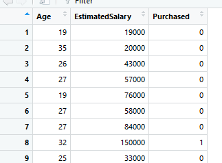
Here is the dataset of few reviews from the customer which is been divided into columns. 1 means the review is positive and 0 means the review is negative.

Cleaning the text

As language is such an integral part of our lives and our society, we are naturally surrounded by a lot of text. Text is available to us in form of books, news articles, Wikipedia articles, tweets and in so many other forms and from a lot of different resources.Majority of available data is highly unstructured and noisy in nature.To 

acheive better insights, its is necessary to play with clean data.The text has to be as clean as possible and here are the steps for cleaning the data:

Removal of Punctuations: All the punctuation marks according to the priorities should be dealt with.  Important punctuations should be retained while others need to be removed

Convert everything to lower case : There is no point in having both ‘Apple’ and ‘apple’ in our data, its better to convert everything to lower case. Also we need to make sure that no words are alphanumeric.

Removing Stopwords : The words like ‘this’, ‘there’, ‘that’, ‘is’, etc. do not provide very usable information and would not want these words taking up space in our database, or taking up valuable processing time.. Such words are called stopwords. It is okay to remove such words with but it is advised to be cautious while doing so as words like ‘not’ are also considered as stopwords (this can be dangerous for tasks like sentiment analysis). For this, we can remove them easily, by storing a list of words that you consider to be stop words. NLTK(Natural Language Toolkit) in python has a list of stopwords stored in 16 different languages.

Stemming : Words like ‘loved’, ‘lovely’, etc are all variations of the word ‘love’. Hence, if we will have all these words in our text data, we will end up creating columns for each of them when all these imply (more or less) the same thing. To avoid this, we can extract the root word for all these words and create a single columns for the root word.

Step2: 

In the above code section we have created a for loop which traverses all 1000 reviews from the customers and acccordingly executes the above steps mentioned and we can see in the corpus vector which is the above output,the reviews have only relevant words which are required.

Bag of words model

A problem with modeling text is that it is messy, and techniques like machine learning algorithms prefer well defined fixed-length inputs and outputs.Machine learning algorithms cannot work with raw text directly; the text must be converted into numbers.It is called a “bag” of words, because any information about the order or structure of words in the document is discarded. The model is only concerned with whether known words occur in the document, not where in the document.

This can be done by assigning each word a unique number. Then any document we see can be encoded as a fixed-length vector with the length of the vocabulary of known words. The value in each position in the vector could be filled with a count or frequency of each word in the encoded document.

Step 3 : 

In this step we construct a vector, which would tell us whether a word in each sentence is a frequent word or not. If a word in a sentence is a frequent word, we set it as 1, else we set it as 0.

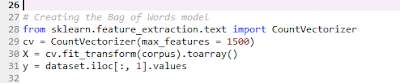
The CountVectorizer provides a simple way to both tokenize(Tokenizing separates text into units such as sentences or words) a collection of text documents and build a vocabulary of known words, but also to encode new documents using that vocabulary.

The max_features attribute sets 1500 relevant words out of 1565 words because  we do not need to use all those words. Hence, we select a particular number of most frequently used words.Further we also create independent variable to be used in the prediction using a machine learning model.

Step 4: Selection of model

The most accurate model for training and test this dataset is from classsification models.Generally for NLP models like random forest,naive bayes,decision tree are the common models used.The model used below is Naive bayes since  the accuracy of the model is much better as compared to other classification models.

In the above confusion matrix there are 55+91 correct predict outcomes whereas rest is incorrect.The accuracy of model turns out to be 71% . Since we had 800 reviews for training set and 200 for test set, so if the number of  reviews was more in training set then the model could easily predict less incorrect values and the model could more accurate.

Thanks for reading!!!

Classification-Logistic Regression

                                                 

                        

  LOGISTIC REGRESSION

Logistic Regression is a Machine Learning classification algorithm that is used to predict the probability of a categorical dependent variable. In logistic regression, the dependent variable is a binary variable that contains data coded as 1 (yes) or 0(no).It is a special case of linear regression where the target variable is categorical in nature. It uses a log of odds as the dependent variable.

Linear Regression Equation:

 y= b0 + b1X1 +b2X2 +......bnXn

Where, y is dependent variable and X1, X2 ... and Xn are explanatory variables.

Sigmoid Function:

                                               p=1/1+e^-y

Apply Sigmoid function on linear regression:

                                  

    p=1/1+e^{-(b0 + b1X1 + b2X2……bnXn)} 

In order to map predicted values to probabilities, we use the sigmoid function. The function maps any real value into another value between 0 and 1. In machine learning, we use sigmoid to map predictions to probabilities.

 Deciding  the boundary:

Our current prediction function returns a probability score between 0 and 1. In order to map this to a discrete class (true/false), we select a threshold value  above which we will classify values into class 1 and below which we classify values into class 2.

p≥0.5,class=1

p<0.5,class=0

For example, if our threshold was .5 and our prediction function returned 0.7, we would classify this observation as positive. If our prediction was 0.2 we would classify the observation as negative. For logistic regression with multiple classes we could select the class with the highest predicted probability.

Building logistic regression in python

To build Logistic regression we consider the following dataset

The dataset contains information of users of a social site.It contains user_id ,gender, age, salary.It has several business clients who can display their advertisement on the social site. One of the clients is a car company who has just launched a luxury SUV for very high price.We will be trying to see which user is going to buy SUV.We are going to build a model which can predict whether the user can buy the luxury SUV.

Step1: Importing the dataset:

Output:

The dataset consists of following columns from which the prediction is based on only two variables  Age and Estimated salary.We will find correlations between Age and salary and the decision to purchase.We are excluding other variables for simplicity in visualization.

Step 2:Splitting the dataset into training set and test set

Step 3:Applying Feature scaling  to the dataset:

Step 4:Fitting logistic regression model in training set and predicting the test set results

Step 5:Generate confusion matrix.

A confusion matrix is a summary of prediction results on a classification problem.The number of correct and incorrect predictions are summarized with count values.It allows easy identification of confusion between classes e.g. one class is commonly mislabeled as the other.

It gives us insight not only into the errors being made by a classifier but more importantly the types of errors that are being made.

Step5: Visualizing the training set results

Output:

Step6: Visualizing test set results

Output:

As seen in the above two graphs of training set and test set,the graph tells us about the users who bought SUV or not.The red users(dots) denotes users who didn't purchase SUV and green users who purchased SUV.Each user is characterized by its age and estimated salary.However in the graphs there are some predictions which turn out to be wrong i.e the green dots on the red region and vice-versa.This amount of incorrect is bound to happen and the number of incorrect and correct predictions can also be identified by confusion matrix.

So, main goal of building this model is classifying the right users into right category.The line between the two classes is the best fit classifier for this model.

Thanks for reading!!!

Polynomial regression

                             

 POLYNOMIAL REGRESSION

Linear regression is the relation between the dependent variable and the independent variable to be linear. If the distribution of the data becomes more complex then the linear line won't best fit in the data. So for the line or a curve to best fit the data we use polynomial regression.How can we generate a curve that best captures the data?

The basic goal of regression analysis is to model the expected value of a dependent variable y in terms of the value of an independent variable x. In simple regression, we used following equation 

                     

                    y=a + bx

Here y is dependent variable, a is y intercept, b is the slope.

In many cases, this linear model will not work out.The predicted results sometimes generate a value which is far from actual values which can lead to wrong information being conveyed.In such cases we use the following equation
   y= a + b1x + b2x^2 +....+ bnx^n

Polynomial regression is a form of regression analysis in which the relationship between the independent variable x and the dependent variable y is modelled as an nth degree polynomial in x

.

Notice that Polynomial Regression is very similar to Multiple LinearRegression, but consider at the same time instead of the different variables the same one X1, but in different powers; so basically we are using 1 variable to different powers of the same original variable.

For example:Consider that there is a  human resource team working for a big company and about to hire a new employee in this company.So the new employee seems to be a good fit for this job and now its time to negotiate about his new salary  for this job.The employee is asking a salary  to be above 160k  annual salary since he has  20+ years of experience and his annual salary was 160k in his previous company. However there is someone in the hr team who wants to know whether the details mentioned by the employee are true or not and that is why the HR retrieves the records of the previous company of different positions.With the help of applying polynomial regression to the above dataset one can find out by building a bluffing detecter to predict whether the analysis leads to truth or bluff i.e whether the new employee had mentioned the correct salary or not. 

To understand polynomial regression,lets generate dataset:

Fitting Linear regression to the dataset:

To implement this in Python we are going to create a LR model first from sklearn.linearmodel and call our object lin_reg

Fit polynomial regression to the dataset:

In this object we are going to call poly_reg that will be our transforming tool which will transform our matrix X in a new polynomial matrix where we can specify the degree we want to run our model with:

Visualizing linear regression results:

We can see that the straight line is unable to capture the patterns in the data.The line signifies the predicted values and the data points are the actual values.The line doesn’t best fits the data and there is huge difference between the actual salaries and predicted which can give a wrong information to the HR.To overcome this we fit a polynomial regression model.

Visualizing Polynomial regression results:

It is quite clear from the plot that the quadratic curve is able to fit the data better than the linear line.The curve best fits the data and the error between the predicted curve and actual curve has decreased which will help  the HR to get correct information about the new employee salary which is approximately equal to 160k annual salary and hance the mentioned details by the employee is correct.

Thanks for Reading!